Introduction

layout: post title: “Theories1” categories: Math —

So far In this writing I have covered

GAN
RNN
Attention
Normalizing Flows
Distributions
Word2vec

GAN math

I am covering some of the GAN maths from my old notes.

The informative PDFGan math1

Recurrent Neural Network

RNN learns while training and remember things learns from prior inputs while generating outputs.

$Output = f(input, hiddenstate)$

RNN takes Series of input to produce a series of output vectors (No preset limilation on size).

Output $o^t = f(h^t ;\theta)$ hiddenstate

$h^t = g(h^{t-1},x ;\theta)$

Unrolled Version,

Optimization algorithm: Back propagation through time (BPTT). Faces vanishing gradient problem. Parameter sharing

Deep RNNs

Bidirectional RNNs

Recursive Neural Network

Encoder Decoder Sequence to Sequence RNNs

LSTM Modified form of RNN to avoid vanishing gradient.

An elaborate tutorial with equations.

A step by step tutorial of LSTM

Understanding the diagram

Another nice tutorial from Roger Grosse source.

Attention

This writing consists of the personalized summary of Attention blog by Lilianweng. Great writer, a personal inspiration. Hope to put my understanding along with his contents.

The primary problems with the seq2seq models are the context vectors limitation.

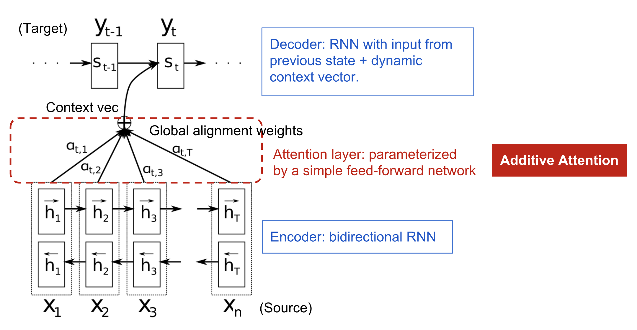
Figure: Source By Bahdanau et al., 2015

Three key points to remember

There is an context vector decides on hiddenstates of encoder
Hidden states weights decides context vector which is calculated by score function and softmax. This calculation leads to a family of context vectors.
Previous state, output and context vector determine next ouput.

Here are some keywords and terms we should distinguish with each other

Self attention: Correlation between current words and previous words
Soft vs Hard attention- Types of weights distribution over the patches
Global vs local:

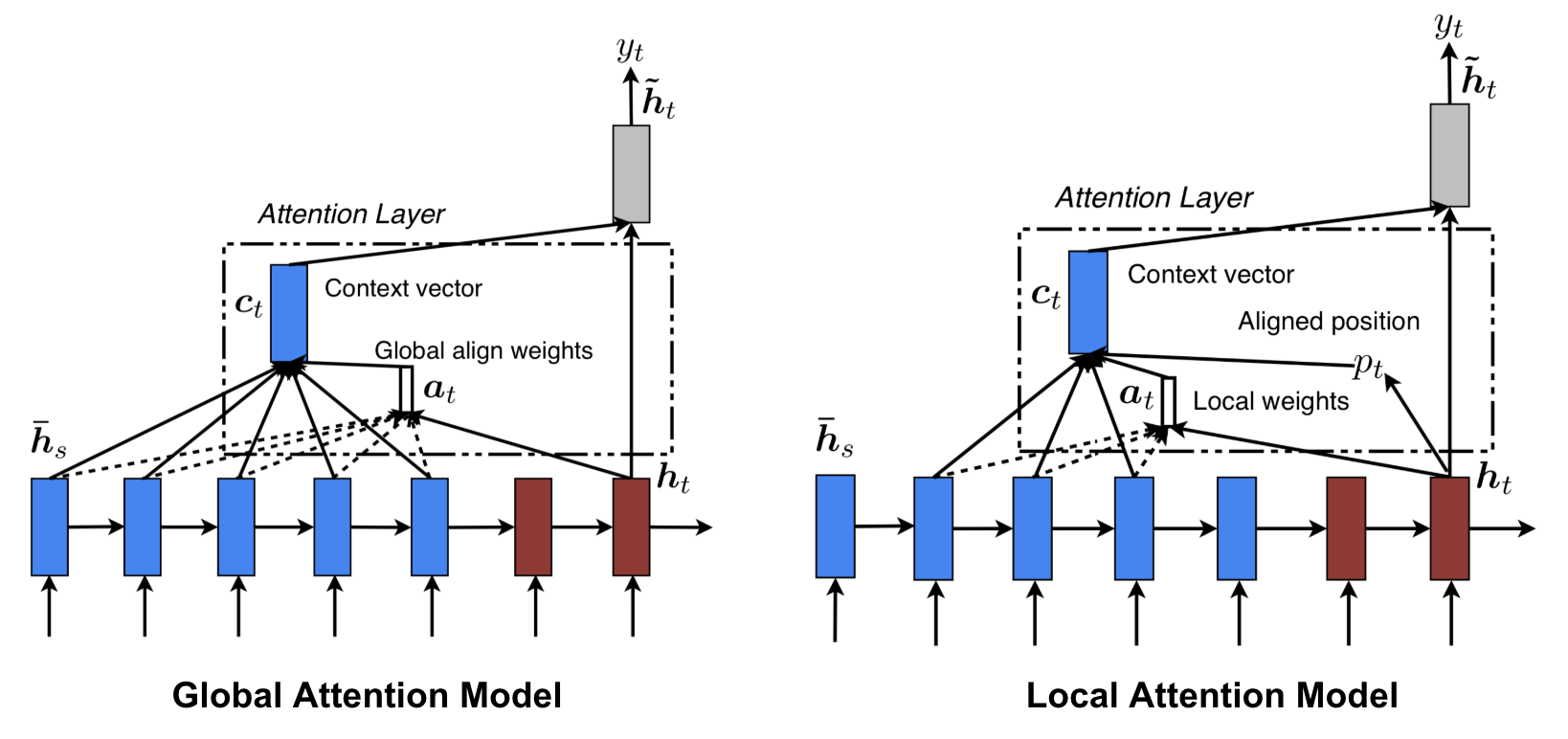
Figure: Global vs local attention source from Luong, et al., 2015

Neural Turing Machine

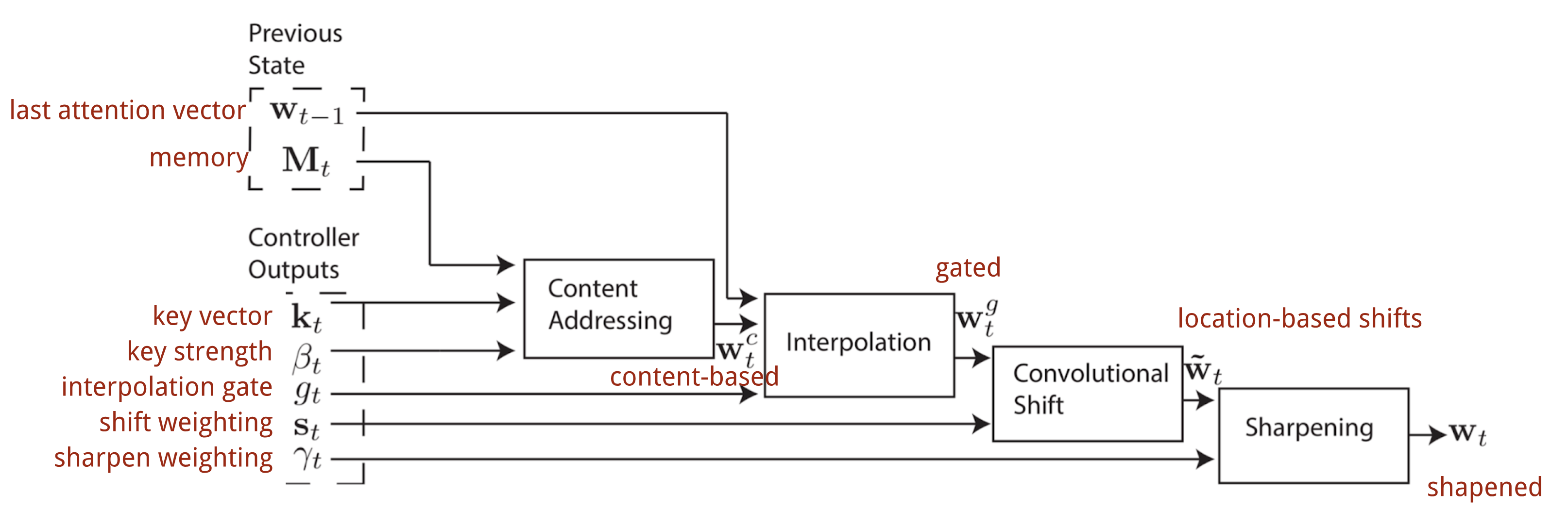Figure: NTM addressing mechanism from Source

Transformer

Seq2seq without recurrent unit. The model architectures are cleverly designed

Key, value and query: Scaled dot product attention. The encoding of inputs are represented by Key Value pairs (V, K). In the decoder the previous output is compressed into a query (Q).

$Attention(Q,K,V)=softmax(QK^T/\sqrt{n})V$

Multi-Head Self-attention

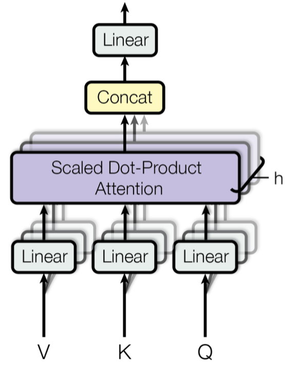
Figure: source vaswani, et al, 2017

Here the key point is the weighting of the V,K, Q to get the final attention.

Encoder Structure

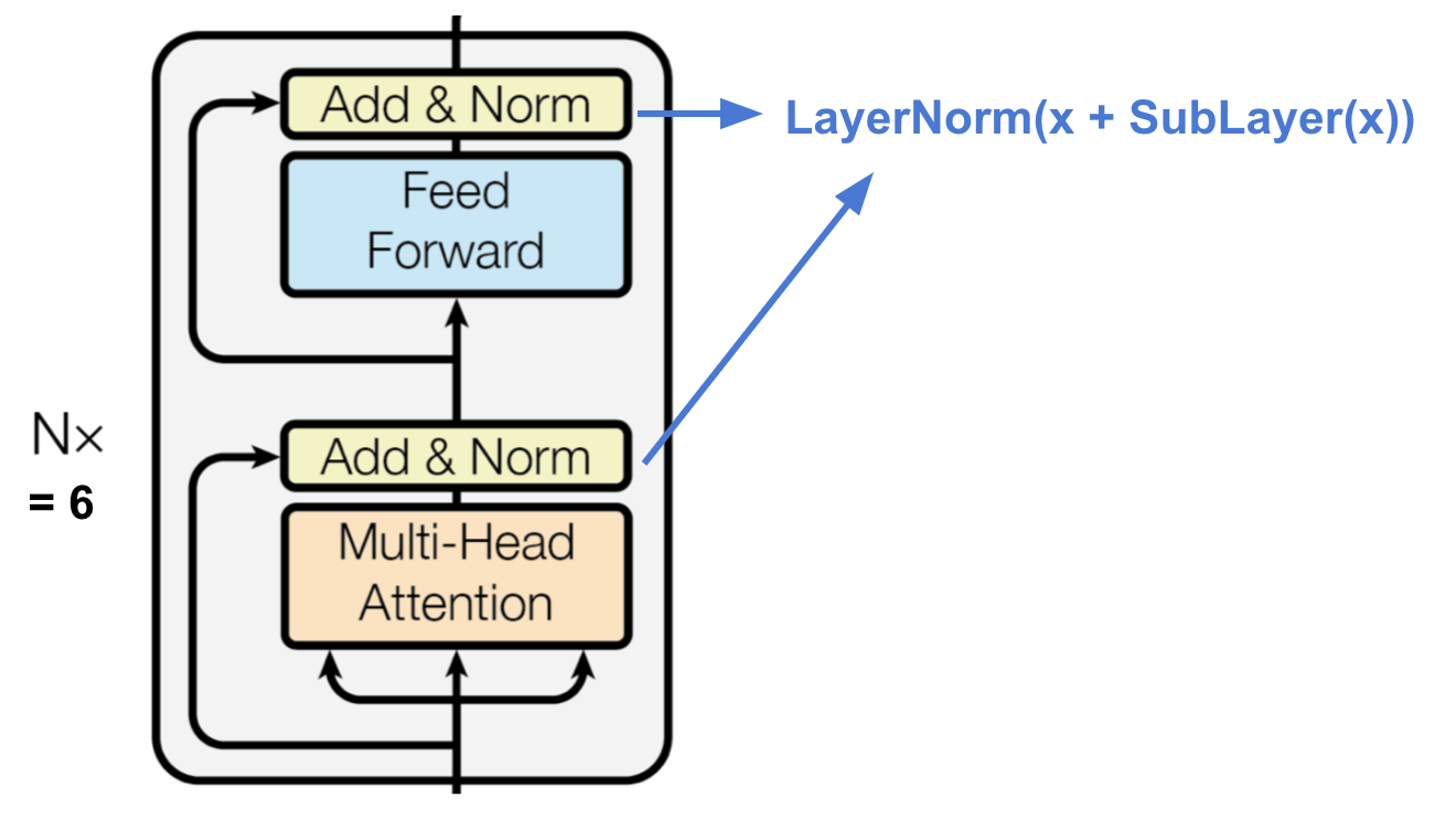
Figure: Source Vaswani, et al., 2017

Decoder Structure

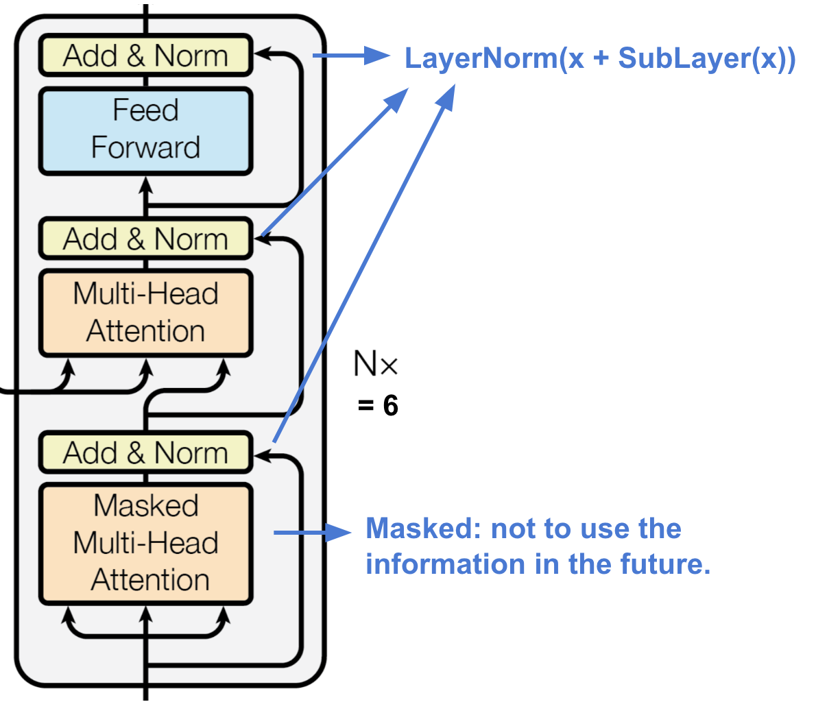
Figure: Source Vaswani, et al. 2017

Final architecture

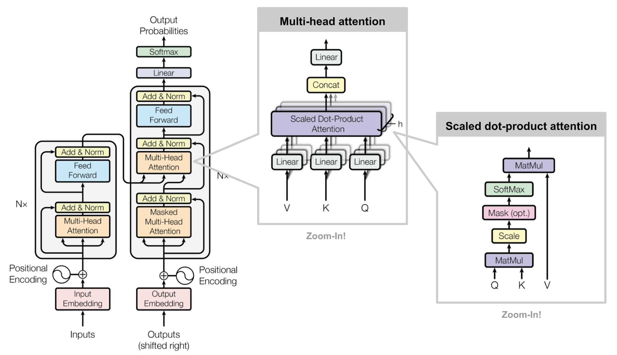
Figure: Source Vaswani et al., 2017

SNAIL

Solves the positioning problem in the transformer models.

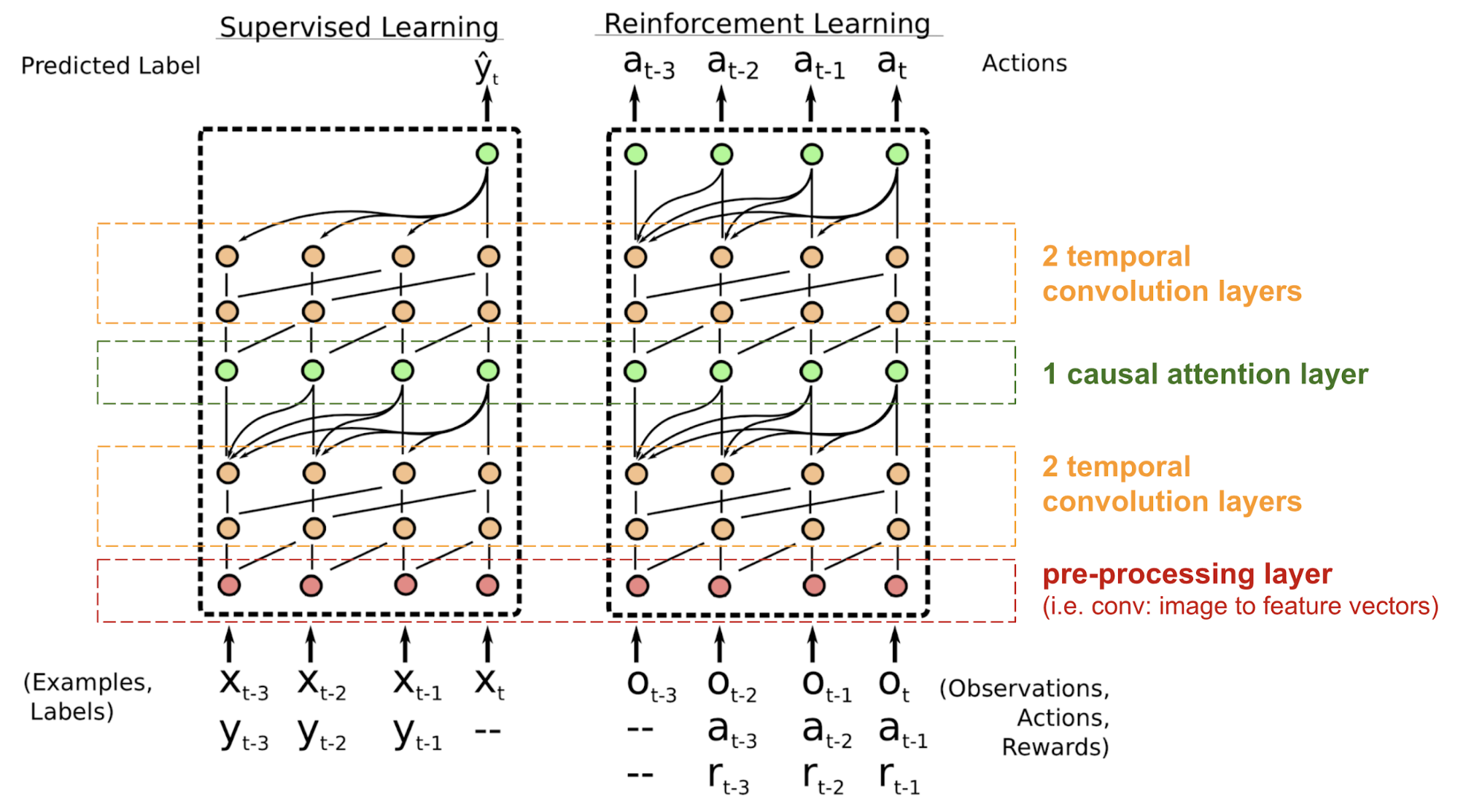
Figure: Source Mishra et al., 2017

Self-Attention GAN

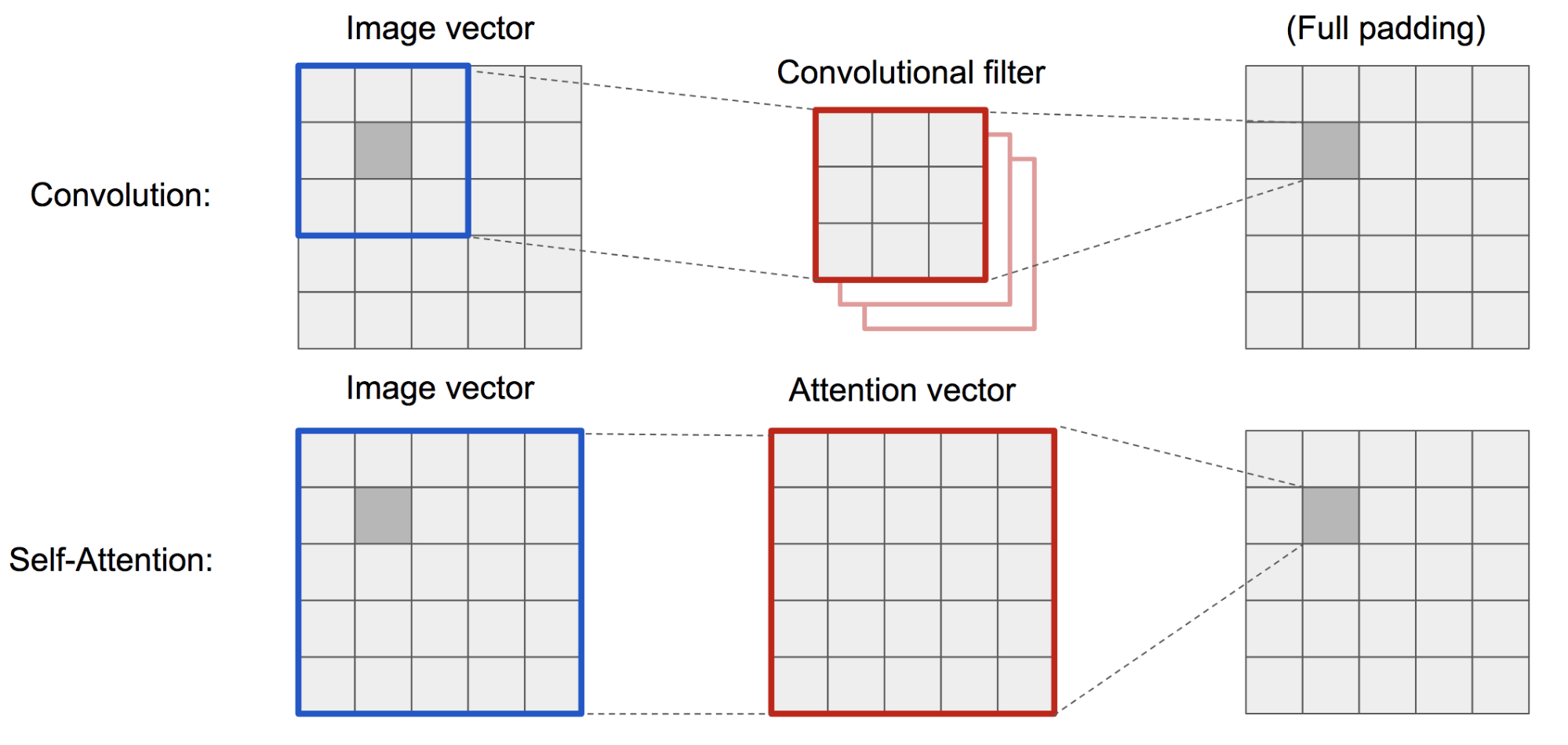
Figure: Convolution operation and self-attention Source Zhang et al. 2018

It has similar concept like key, value and query (f, g, h).

Figure: Self-attention source Zhang et al., 2018

Normalizing Flows

Motivational blog1 and blog2

More motivational blog

Problems with the VAE and GAN- They don’t explicitly learn the pdf of real data as $p(x)=\int p(x|z)p(z)dz$ is intractable to go through all latent variable z. Flow based generative model overcomes this problem with the technique normalizing flows.

Types of Generative models

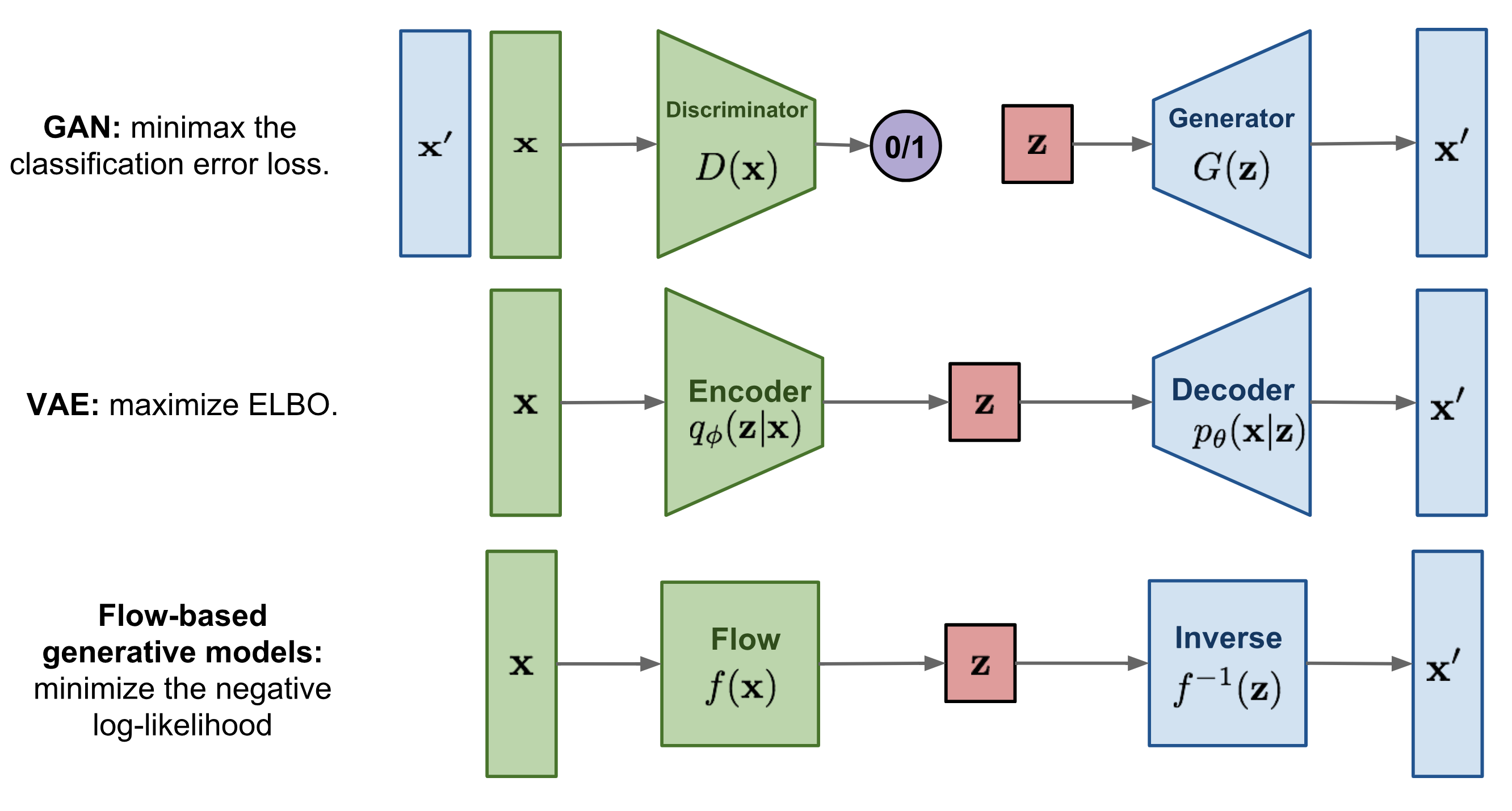
Figure: sources

Normalizing flows are techniques to transform simple distribution to complex distribution. This ideas are entangled with the invertible transformation of densities. These transformation combinely forms Normalizing Flows

Figure: Source

Here assuming,

$z_{i-1}\sim p_{i-1}(z_{i-1})$ and $z_{i}=f_i(z_{i-1})$

so, we find

$\log{p_i(z_i)}=\log(p_{i-1}(f^{-1}(z_{i}))+\log{det(J(f^{-1}(z_i)))}$

Expanding total form

$X=Z_K=f_k.f_{k-1}....f_1(z_o)$

Becomes

$\log{X}=\log(p_o(z_{0}))+\sum_{i-1}^K\log{det(J(f^{-1}(z_i)))}$

In short, the transformation random variable $z_i=f_i(z_{i-1})$ goes through is the flow and full chain is the normalizing flows.

Estimating parametric distribution helps significantly in

1. Generate new data
1. Evaluate likelihood of models
1. Conditional distribution estimation
1. Score the algorithm be measuring entropy, MI, and moments of distribution.

There has been lack of attention in the (2., 3. and 4.) of the previous points.

The Question is to feasibility of finding distribution with following properties:

Complex and rich enough to model multi-modal data analysis like images/value function
Retain the easy comforts of Normal distribution!

The solution is:

Mixture models with re-parameterization relaxation.
Autoregressive factorizations of the policy/Value function
In RL symmetry breaking value distribution via recurrent policies, noise or distributional RL
Learning Energy-based models - Undirected graph with potential function.
Normalizing Flows - learning invertible, volume tracking transformation for distributions to manipulate easily.

Change of variables, change of volume

Lets go over some points

Linear transformation of points is a spacial case of y=f(x); x, y are high dimensionals vectors (We will talk about f(x) in general as transformation)
PDF and CDF
Jacobian, Jacobian of inverse function and Determinant - Change in volume by transformation.

Consider x as Random variable and

$x=f(y)$

Now PDF $p(y)=p(f^{-1}(y)).det(J(f^{-1}(y)))$ Taking log $\log{p(y)}=\log(p(f^{-1}(y))+\log{det(J(f^{-1}(y)))}$

Models with normalizing Flows

Simply the negative log likelihood of the data

Real-NVP (Non-volume preserving)

Another recent network; Affine coupling layer.

first 1:d stays same
d+1:D undergoes affine transformation.

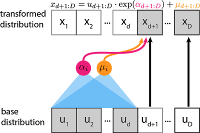
Figure: Special case fo the IAF as 1:d in both x and u are equivalent. Source

NICE

same as real-nvp but the affine layer has only shift (sum)

Glow

Activation layer
Invertable 1x1 conv layer
Affine coupling layer

Figure: Sources

Autoregressive Models are Normalizing Flows

A density estimation technique to represent complex joint densites as product of conditional distributions.

$p(x_{1:D})=\prod_ip(x_i|x_{i-1})$

For common choices, we have

$p(x_i|x_{i-1})=\mathcal{N}(x_i|\mu_i,\exp(\alpha_i)^2)$

Where,

$\mu_i=f_{\mu_i}(x_{1:i-1})$

and

$\alpha_i=f_{\alpha_i}(x_{1:i-1})$

Here the inductive bias tells that earlier variables don’t depend on later variables! To sample from the distribution to get data x from 1:D

$x_i=u_i\exp\alpha_i+\mu_i$

where $u_i from \mathcal{N}(0,1)$

Now,

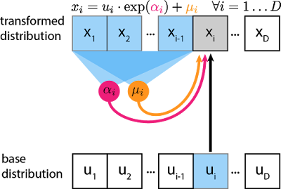
Figure: Graphical View source

Here the learnable parameters are alpha’s and mu’s by training neural network with data. and the inverse

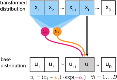Figure: Earlier Source

MADE

Uses autoregressive property in a autoencoder efficiently

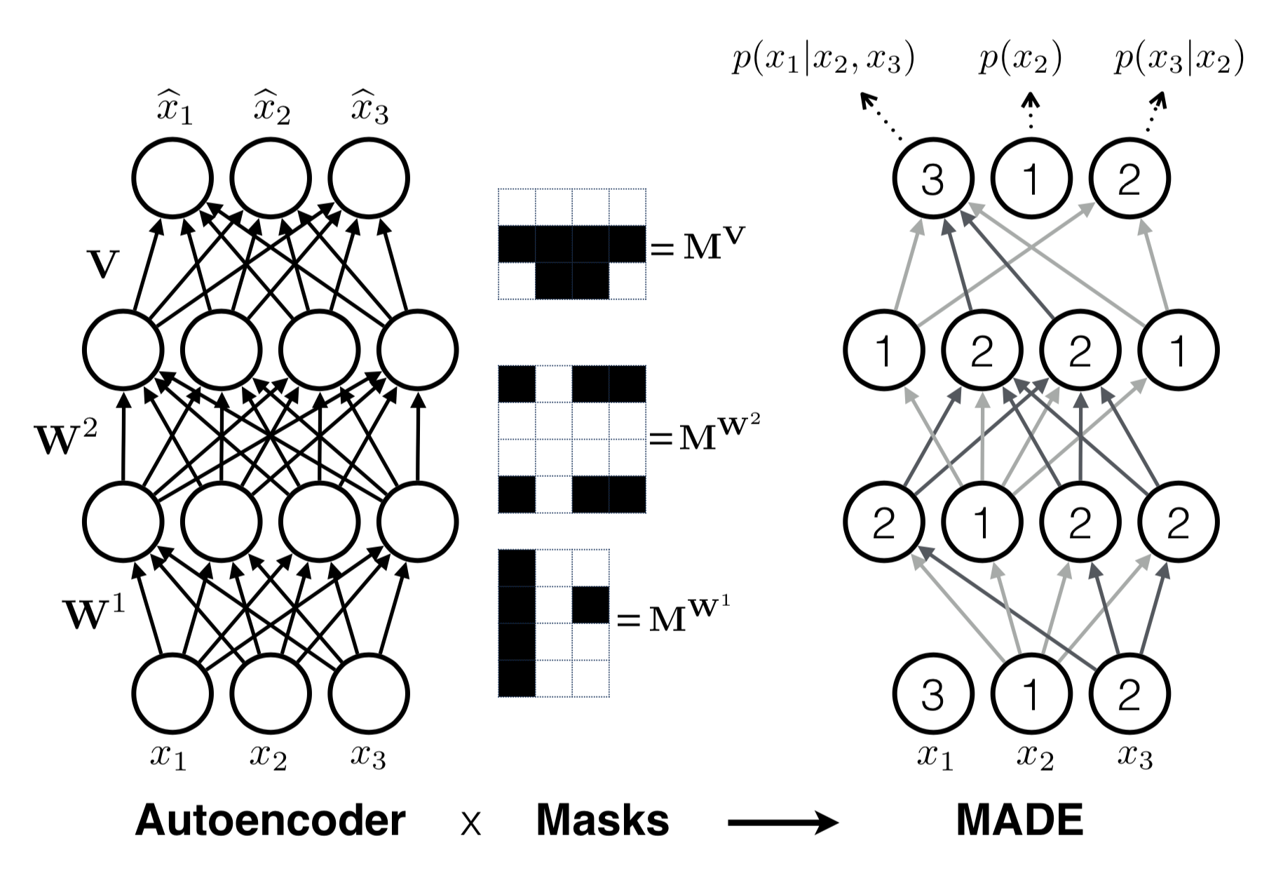
Figure: Source

PixelRNN

Pixel generated on condition of earlier pixels
Uses visual attention

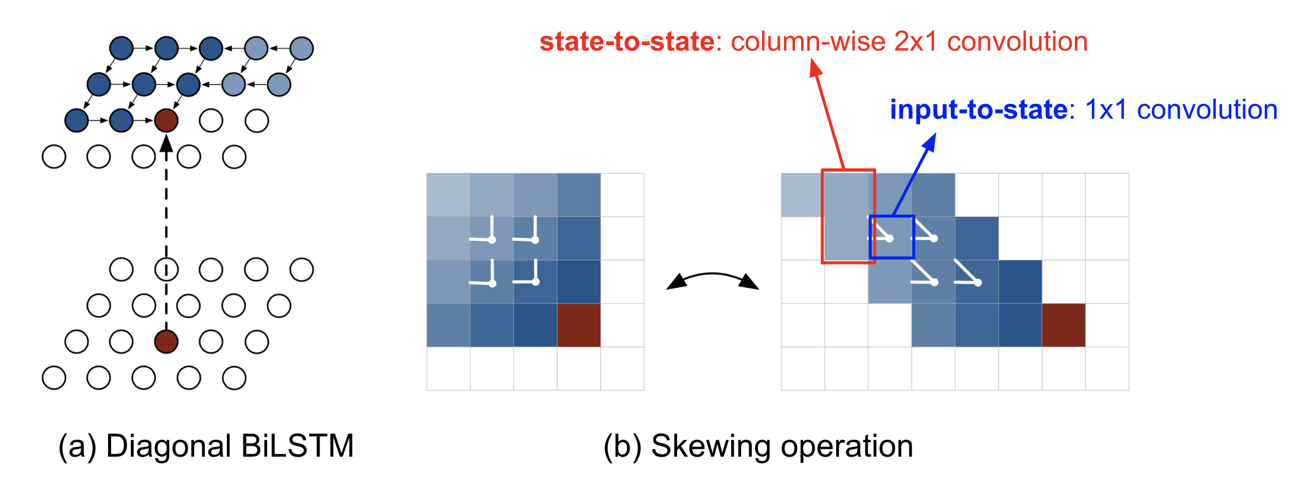
Figure: Source

WaveNet

PixelRNN applied to Audio Signal

Figure: Top diagram shows Wavent and bottom picture shows the causal convolutional layers Source

Inverse Autoregressive Flows(IAF)

Two major change in equations from the Masked AF earlier

$p(x_i|x_{i-1})=\mathcal{N}(x_i|\mu_i,\exp(\alpha_i)^2)$

Where,

$\mu_i=f_{\mu_i}(u_{1:i-1})$

and

$\alpha_i=f_{\alpha_i}(u_{1:i-1})$

Mind the disinction between u and mu

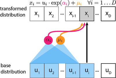
Figure: Source Looks like inverse pass of MAF with changed labels. Extract u’s from the x’s using alpha’s and mu’s.

MAF (trains quickly but slow sample) and IAF (trains slow but fast samples) are trade of each other.

Masked Autoregressive Flows

Similar to IAF - but introduced earlier.
Goes from one known distribution to another

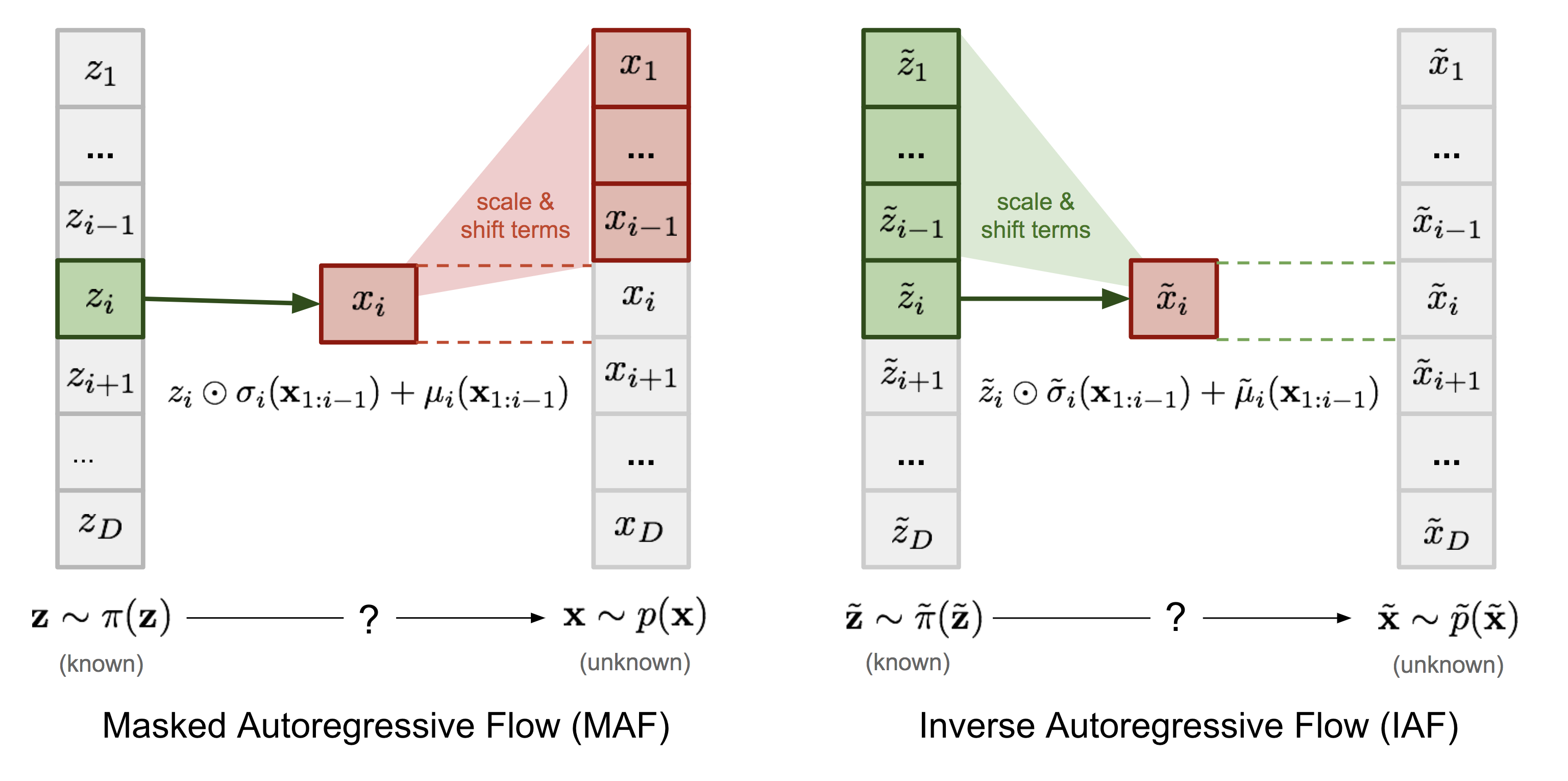
Figure: Difference between MAF and IAF. I believe, the IAF equation should be z instead of x in the transition. source

Parallel Wavenet

Combination of MAF and IAF is done in Parallel wavenet. It uses that idea that IAF can compute likelihood of own data cheaply but not for external data. MAF learns to generate likelihood of the external data.

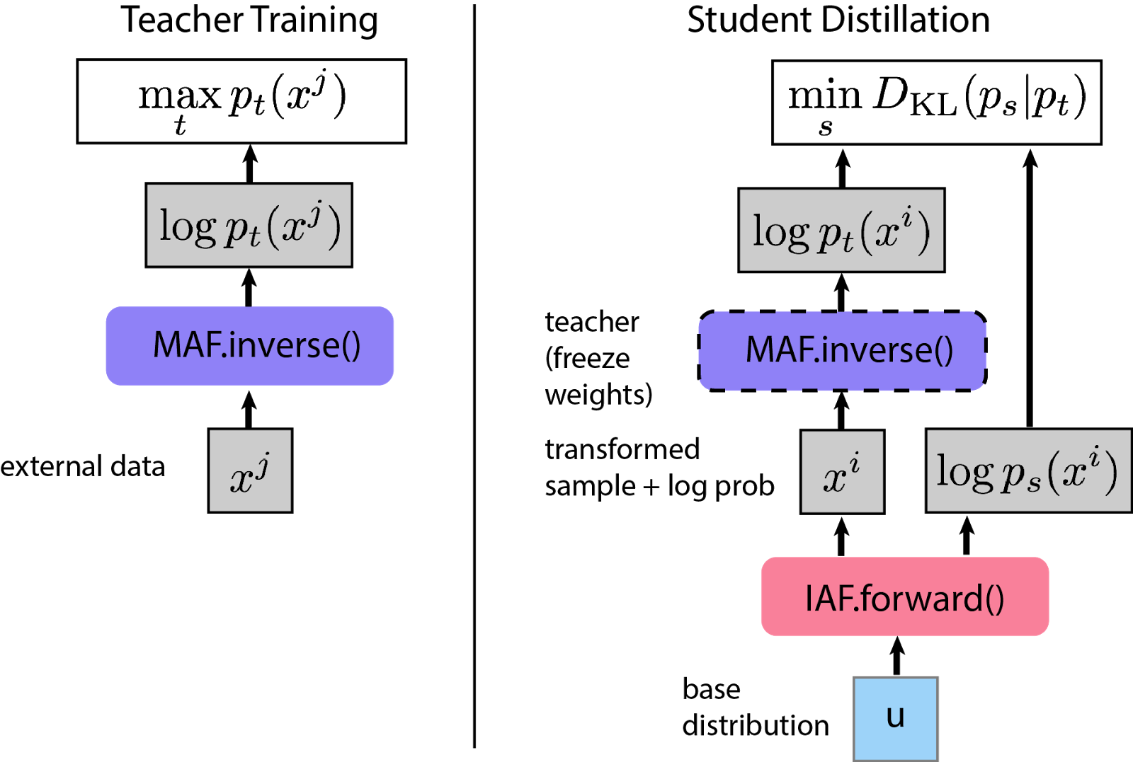
Figure: Source Here MAF (teacher) trains to generate samples and IAF (student) tries to generate samples with close match with teacher’s likelihood of the IAF generated samples.

Distribution

Probabilities and machine learning are more than connected. In ML we need to have a clear understanding of the Probabilities, distribution, densities and how they are connected with each others.

Here is my short note

And another big notes not by me

Word2vec

Elaborate explnation

Gradient, Hessian, Jacobian

good cover

Simple things but comes back to increase you confusion again and again. They all comes with the functions of variable and their derivatives but in vector/matrix form. Lets dive into gradient first. Gradient (delta) is integrated with multi-variable to single value [Rⁿ to R] function and partial derivatives. Hessian (delta square) just follow the definition of gradient to second order. Gradient covers the slope of f with each variables. Hessian looks into the second derivatives w.r.t each variables. Hessian matrix have partial derivates of function with each of the two variable combines.

Now the jacobian is defined for multi-variable to multi-function [Rⁿ to R^m]. Matrix of derivative of each function with each variable once. Jacobian is basically defined for the first derivative of the functions.

Now if we think gradient as a multivariable to multi function then jacobian of it [gradient vector function] is the hessian of the original function f.

The key point to remember is vector valued and scale valued function for multiple variables. intersting and connection to Laplacian.