Probabilistic Terminology

Two very important laws: Law of total probability and law of total expectation.

Entropy:

Distribution Alert!!!

Well look at that Beautiful equation till it satisfies the eye and mind.It gives a value [point estimation]. Two things to remember when talking about an Entropy. 1. Probability distribution (Think of PDF; sum constraint to 1) and 2. Expectation of Log of the distribution over the allowed range. BooM. We get entropy!. Of course negate it. As log of something less than one is negative.

Special property: Given a PDF, Expectation log of that PDF is minimum if we take expectation w.r.t. the PDF itself. A.k.a cross entropy of q(x) w.r.t. p(x) distribution [notion of cross entropy]. This doesn’t provide anything on the limit of the entropy of q(x).

Some important things to remember

• H(f(X)) <= H(X); Known function doesn’t reduce entropy.
• H(X,Y) <= H(X) + H(Y); Worst case the maximum entropy of x and y can be summed.

Conditional Entropy The above may give a vibe about negative of KL divergence but it’s 100% not KL divergence. As the p(x) is not a probability distribution over x,y [doing the summation math over x-y space p(x) may be well over 1; crap! This breaks the PDF constraint!] space but only over x. This changes everything as the ratio p(x,y)/p(x) is always less or equal to 1 [p(y:x)]. Please refer to mutual entropy for more clearance. p(x)p(y) is a distribution over x-y space [doing the math of sum over x,y; combinatorial multiplication of p(x)p(y) over the x,y space], so does p(x,y).

Conditional entropy provides the entropy that knowing the conditioned variable won’t reduce. H(X:Y) [: sign to mean condition in this text] means how much entropy still remains for X given we know Y. It can be maximum of H(X) (independence) and minimum to 0 (certainty). H(X) contains sum of two distinct parts 1. MI and 2. Conditional entropy. This is expectation of logP(x:y). The conditional probability p(x:y) may increase or decrease from p(x) but the H(X:Y) will decrease or at max stay the same as H(X).

Some useful points (think of Venn diagram)

1. H(Y:X) = H(X,Y)-H(X) = H(X:Y) + H(Y)-H(X); Subtract the known information from the Total unknown
2. H(Y:X) <= H(Y) ; Knowing something can’t increase the entropy.
3. H(Y,X) = H(X) + H(Y) - I(X;Y) ; Refer to MI section
4. H(Y:X) = H(Y) in case of independence

Cross Entropy Cross entropy of distribution q(x) w.r.t distribution p(x) is always greater than entropy of p(x) [discussed earlier]. Whatever distribution is inside log() that’s entropy we are calculating. We are just introducing more uncertainty! Cross entropy is minimum when p(x) and q(x) are same for all x, which is equal to entropy of q(x) or p(x) given, setting the kl terms to 0 by equating p and q distributions. Cross entropy provides a higher bound on entropy over p(x), nothing to do with entropy of q(x)[-log q(x) expected w.r.t q(x)], it can be 0 or very high though.

The key focus upon the p(x) [which distribution is using for entropy calculation], as cross entropy w.r.t. p(x) would allow to know the higher bound of entropy of p(x). Knowing H(p,q) we know the upper bound for the H(p) and vice versa. {discussed above}

entropy comparison: who is what

Renyi Entropy

properties

Mutual Information

From Wikipedia:

or

This notation of joint entropy [H(X,Y) = E[log p(x,y)] w.r.t. distribution of p(x,y)] may be confused with the cross entropy H(p,q). Joint entropy takes two RV where as the cross entropy takes two distribution over the same RV.

This is another important and insightful equation with insight. The MI tells us mutual unknown between x and y together. Think of Venn diagram. MI indicates the region where both x,y intersects in terms of unknown. Alternatively, if we know x how much it helps to understand y, or vice versa. Since if we knew is there, this is still uncertain. MI is basically how much entropy is reduced by knowing X or Y from the total entropy of Y or X, commonalities between them! So it has to be lower or equal to the entropy of X or Y. Bound of MI is 0 to min(H(X), H(Y)). The higher the better from info gain perspective.

Quick derivation: If p(x), p(y) are independent the then there is no mutual information or MI=0, [Basic p(x,y)=p(x)p(y), in case of independence]. MI upper bound is minimum(H(x),H(y)); one is described by the others totally.

Some Useful points

1. I(X;Y) = H(Y) - H(Y:X); Subtract the conditional entropy (unknown) from the total entropy (unknown), leaving how much we know about them simultaneously.
2. I(X;Y) = H(X) -H(X:Y)
3. I(X;Y) = H(X,Y) - H(X:Y) - H(Y:X)

Kullback-Leibler (KL) Divergence

Another commonly encountered term. Can be expressed as cross entropy of q w.r.t p and entropy of p terms (subtraction.). This can be interpreted as entropy overestimation by selecting log q instead of log p with both expectation w.r.t distribution p. As discussed above knowing E[-logq] w.r.t p we already know the upper bound for E[-logp]. Clearly minimum to 0 in case of p and q are same for all x.

Quick points: This is not a metric as it’s not symmetric. This is in coherence that E_p[logq] has nothing to do with E_q[logq] (Upper bound for E_q[logp]). [QuickNote: Look and understand the sign. E_p[logq] is lower bound for E_p[logp]; But E_p[-logq] is the upper bound for E_p[logp], so does the other combinaortial options.]

Two interesting view of the KL divergence link

more into it link

• Supervised Learning (forward KL) - arg min D_KL(P||Q_theta) Mean seeking behavior; where p is high, Q must be high. [less penalty for low point missing of P by Q]. Calls zero avoiding behavior Q should get P by mean [get all the high point for the P modes in expectation ]
• Reinforcement learning (Reverse KL) - arg min D_KL(Q_theta||P) Mode Seeking behavior; Where Q is high P must have high too [less care when Q is low] - get the maximum mode for the P by Q. (as the equation log(value) multiplied by Q), So Q will place itself to get the maximum mode of P. calls zero forcing behavior.

Another cool format

Don’t confuse it with the conditional formula, that one was joint distribution. The uncertainty (Loosely entropy) will increase or at least stay same, meanwhile for conditional the uncertainty will decrease or at maximum stay same. Moreover conditional entropy has two RV and here is only one but two distributions.

Very much related to fisher information metrics. In another day math

Generalized formula:

properties

f-divergence family

From Wikipedia

f-divergence to other Divergence

Divergence	corresponding f(t)
KL-divergence	t*logt
Reverse KL	-logt
Total variation distance	.5*abs(t-1)

Bregman divergence

Maximum Likelihood

MAP

Expectation Maximization

nice post another one

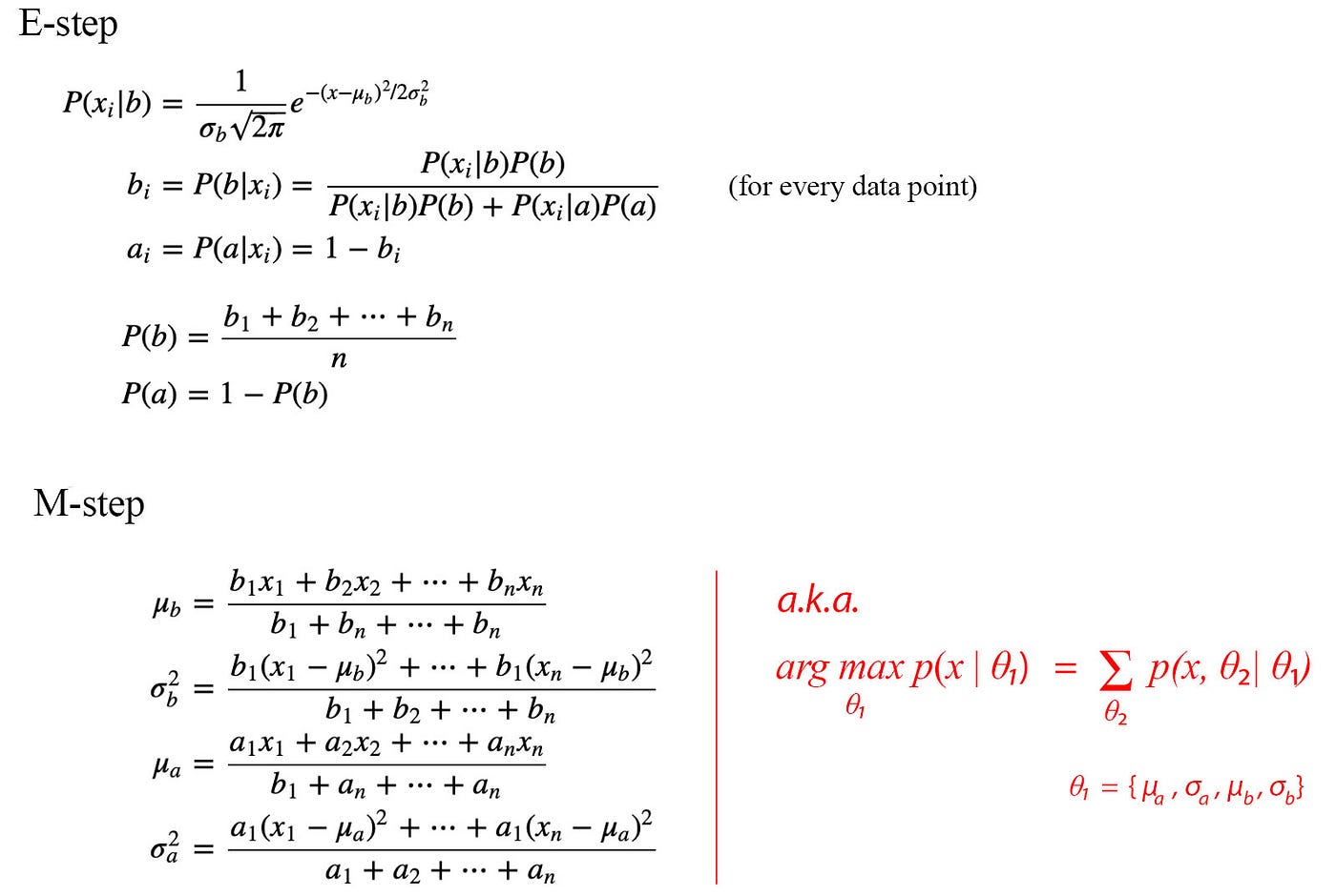Figure: From source very intuitive

Evidence Lower Bound

Nice intuitive link

This provides lower bound on logP(X) given the all data point observation X and an approximation of parametric distribution. It’s always negative or at max 0. This bounds the log likelihood of data observation.

Two alternative formulation. One gives the actual bound and other gives the difference of log likelihood and the bound itself, kl of estimation q(z) and true posterior p(z

x). Here we assume the q(z) and the true posterior is unknown or we try to reach.

Always negative.

Banach Fixed point theorem

Well, lets start with Metric space; a ordered pair (A,d)

• A non empty set
• Real valued distance function d: AxA to R, satisfies metric space axioms. for x, y \epsilon A
  • d(x,x)>0
  • d(x,y)+d(y,z)>=d(x,z)
  • d(x,y)= d(y,x)
  • x=/y; d(x,y)>0

Cauchy sequence: for complete metric space

• 

Contraction Mapping:

• function f; from one metric space to another metric space: d2(f(x1),f(x2))<=d1(x1,x2) ; f lipschitz continous with lipschitz constant less than 1

Uff, finally, for complete metric (M,d) space, if f: M to M be a contraction

Then, 0<=q<1: d(f(x),f(y))<=qd(x,y)

Then there are unique fixed point of f : f(x)=x

Norms and Condition Number

nice tutorial Vector norm: l2, l1 ,.. l-infinte norm. Definition. where x_i are the vector elements.

Think of a point in n dimentional space.

Matrix norm in little tricky where x_v symbolizes a vector.

Well this is a maximization. Of course l1 norm would be sum of maximum absolute column value [multiply one hot encoding vector and norm]. l_infine norm would be maximum sum of rows [multiply by all one vector].

Condition Number

Depends on which norm we are considering.

It also means the ratio of maximum and minimum stretching of some vectors proof. Computation is tricky due to matrix inversion operation. For non singular l2 conditional number of a nonsingular matrix would be the ratio of maximum to minimum singular value of matrix. The more close to singular the higher condition number. some extra

EigenValue

power iteration

• Find dominant (if exist) eigenvalue
• Look at the theorem
  • nxn diagonizable matrix with dominant eigenvalue.

diagonizable

• for nxn matrix their is n distinct EigenValues
• If harmitian the all the eigenvectors are orthogonal to each other.

link

Linear algebra Essentials

blog post

Vector scaler product is projection. Matrix multiplied with vector is the projection of vector in each of the row of the matrix. Well simple but very effective!! Just apply it next time we encounter some vector, vector or matrix, vector multiplication.

Combine multiplication with eigenvector value! or orthogonal or parallel.

Markov Random Field

Graph Definition

Lipschitz

LP duality

PSD matrix

One thing that appears again and again. Let’s dive into conceptual plane about what the Positive Semidefinite matrix. Well, simply, this is a property of matrix Norm with symmetry condition. Two things to come immediately with PSD concept

• M is symmetric
• v^TMv >= 0 It follows that when the 2nd condition is always strictly greater than 0 it is call positive definite matrix. and < 0, means negative definite matrix.

As I promised to go beyond the definition, lets break the 1st condition. Hmm, Symmetric Matrix. Row, Columns are same. Lots of other things follow or shorter. What hits me most is the property of eigenvalues for real symmetric matrix (spoiler alert: All eigenvalues are real) and diagonizable by the forming a matrix by taking the eigenvectors as rows [can be written as weighted sum of vector multiplication (nxn)(nxn)(nxn) to nxn shape]. This can be extending to multiplication of two matrix (M=B^TB) by reformulating the diagonizable equation [can be written as weighted (all weight 1) sum of vector multiplication (nxn)(nxn) to nxn shape].

The second condition says, that project (transform) any vector on the matrix rows and project it on the original vector would make it positive or atleast zero. Means projection will not rotate the vector in the opposite direction. This automatically lead the property of the eigenvalues for PSD matrix (yes they will all be always positive), just shrink or expand it but not reverse the eigenvector (or any vector) by definition.
shorthand

more

Symmetric Matrix has real eigenvalues and the eigenvectors are always orthogonal to each other. link1 link2

FID

Use to evaluate Gan generator performance.

Mathematical definition

First let’s start with inception distance.

As the equation states, it measures the distribution entropy of label (y) of the generator from the original. It just look at the label distribution! It should reduce the entropy of label given generated image [means we can understand the object from the generated image easily], label uncertainty reduce. In other words, E_x~gen[-log p(y given x)] should be low. Secondly, the marginal distribution of y given x, w.r.t. x should match the real data label distribution.

The problem is that IS offers no statistical measurement. p(y given x) can be vague in the original image too! Then why we want to reduce it in the generated image. Moreover, p(y given x) can be misleading.

Here comes the FID, [lets assume the multivariate gaussian; yes we have to do it]. Now fit the multivariate gaussian to find the parameters for both the real and the generated image [of course after passing them for some further modification; inception V3 layer activation.]. .

Finally calculate;

As expected the lower the better. They are measured in the inception layers activation map for the real and generated image.

Loss functions

Cross entropy:

Its derivative formula. It’s also related to focal loss.

Hinge Loss:

InfoMax principle:

link

Linear algebra

A orthogonal vector, w.r.t a particular hyperplane, defines the same hyperplane using the dot product with generalized co-ordinate symbols with a bias addition. Mathematically, the hyperplane can be expressed as dot(wx)+b = 0; w (w.r.t the 0 coordinate) is a vector orthogonal to the hyperplane itself. We can rephrase that all the points that form hyperplane, collectively are orthogonal to the vector. This is the interesting parts. For example, x-2y + 1 = 0; can be simplified to w =(1, -2), x= (x,y) and bias term is 1. Now get the point (1,-2) in x-y plane, draw a perpendicular to that line and shift it by 1! Hola, you have your simplest hyperplane in 2 dimension. Now, you may extend it for more dimensions.

By following the idea that dot product is a projection, the hyperplane equation also can be presented by the projection idea. All the points in the hyperplane if projected on the normal vector w, its value will be negative of the bias value.

read more read more 1 read more 2

Conjugate priors and beyonds

Binomial to multinomial

And distribution over distributions

Binomial and multinomial extension of Beta distribution and dirchlet distribution link

conjugate prior - why beta is conjugate for the binomial distribution .

dirchlet is the conjugate prior for the multinomial distribution. - posterior of the probabities given the data is another dirchlet distribution

Beta distribution - Can approximate different distribution you tube link

LDA simplified

HMM

link