Introduction

This blogs contains some of the commonly encountered terms in DL. Lets Move forward. The containing terms are

• Embedding
• Collaborative Filter
• Boltzmann Machine
• Restricted Boltzmann Machine
• Noise contrastive Estimation
• Active Learning
• Encoder

Embedding

Very nice post to start.

• Mapping of discrete variables to latent low dimensional continuous space instead of one hot encoding. 3 motivations
  • Nearest neighbors
  • Input to supervision task
  • Visualization
• Learning embedding- Supervised task to learn embedding.

Collaborative Filter

Boltzmann Machine

courtesy: Hinton

• Search Problem
• Learning Problem

Stochastic dynamics of Boltzmann Machine.

The probabilities of being a neuron to one is

The interesting Collection: if the units are update sequentially independent of the total inputs, the network will reach Boltzmann/Gibbs distribution. (Google it.) Here comes the notion of energy of state vector. It’s also connected to Hopfield network (1982): Described by undirected graph. The states are updated by the connection from the connected nodes. The neural attract or repel each other. The energy is connected with the node values, thresholds and edge weights. The update rule of S_i = 1 if sum of w_ij*s_j > threshold else -1. Following the update rule the energy either decreases or stays same. Different from Hopfield as for the probabilistic approach of weights.

There probabilities of states being in the v energy states. The probabilities of being a neuron to one is where E(v) represents energy function. The probabilistic state value helps to overcome energy barrier as it goes to new energy state sometimes.

Learning rule and update using gradient ascent. <> is expectation. This causes slow learning as the expectation operation. Quick notes- data expectation means: Expected value of s_i*s_j in the data distribution and model expectation means sampling state vectors from the equilibrium distribution at a temperature of 1. Two step process firstly sample v and then sample state values.

Convex: When observed data specifies binary state for every unit in the Boltzmann machine.

Higher order Boltzmann machine

Instead of only two nodes more terms in energy function.

Conditional Boltzmann Machine

Boltzmann machine learns the data distribution.

Restricted Boltzmann machine (Smolensky 1986)

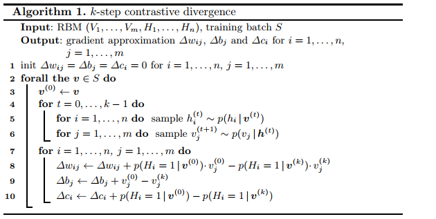
A hidden layer and visible layers: Restriction: no hidden-hidden or visible-visible connection. Hidden units are conditionally independent of the visible layers. Now the data expectation can be found by one sweep but the model expectation needs multiple iteration. Introduced reconstruction instead of the total model expectation for s_i*s_j. Learning by contrastive divergence.

Related to markov random field, Gibbs sampling, conditional random fields.

RBM

Nice post by invertor

Key reminders: Introducing probabilities in Hopfield network to get boltzman machine. Now one hidden layer makes it RBM with some restriction like no input-output direct connection or hidden-hidden connection. One single layer NN.

Learning rule: Contrastive divergence (approximation of learning rule of (data - model))

More cool demonstration for contrastive divergence.

Learning Vector Quantization

Fairly simple Idea. Notes

Its a prototype-based learning method (Representation).

• Create Mean to initialize the vector for each class as initial representation.
• Find Distance for each example
  • Update only for the closest prototype (representation) by some distance metrics.
  • If matches with original class (nearest to the actual class of representation) update the representation to go near the example
  • If not agrees than the representation is updated to move away from it.
  • Repeat for each examples to complete epoch1

Noise Contrastive Estimation

original Paper

Contrastive loss:

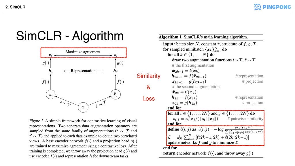
link 1 The idea that same things (positive example) should stay close and negative examples should be in orthogonal position.

• SimCLR ideas

link 2

link 3 Same ideas different applications.

initial paper with algorithm with a simpler explanation resource.

concise resource

Triplet loss training tricks

some loss function to formulate

• Max margin losses
• Triplet loss
• Multi-class N-pair loss
• Supervised NT-Xent loss

visual product similarity - Cornell

Some notes on Recent review

• Property of representation - Distributed, invariant and disentangled
• What is contrastive learning
  • Representation learning
    • Generative and Discriminative Models
    • Supervised and unsupervised learning
    • Objective and Evaluation of Representations? Interesting
  • Contrastive representation learning
    • Learning by comparing
  • Instance discrimination
    • Figure 2
    • Feature Encoders (Body)
    • MLP heads (Projection layer) [discarded after training]
    • Loss function itself
  • CL taxonomy
    • Figure 3
    • Data taken from p(k,q) distribution instead of the P(x) distribution [see the description if needed]. In practice quiry is sampled first the positive and negative keys.
    • Models and encoder, transformer head and losses.
    • Figure 5 [interesting notion of the similarity]
  • Notable works
    • multisensors -Time contrastive network
    • Data transform
      • SimCLR
    • Context-instance relationship
      • Deep InforMax
      • Contrastive predictive coding
    • Sequential coherence and Consistency
      • Figure 8 [multiframe TCN]
    • Natural Clustering
      • Metric learning
      • Prototypical Constrastive Learning [??]
      • SwAV
    • Taxonomy of the encoders
      • End to end
      • Online offline encoder
        • MoCo
        • Memory bank
      • Pre-trained encoder
        • BERT (!)
        • Distillation (Contrastive representation distillation)
    • Head Taxonomy
      • Projection Head
      • Contextualization head [context-instance relationship (section 2) - Aggregate multiple heads together]
        • Contrastive Predictive Coding
        • Deep InfoMax
      • Quantization Head (!) [Map multiple representation into same representation]
        • SwAv
    • Loss Function Taxonomy [interesting ]
      • minimize distance between pairs but problem with collapse
        • Negative pair or architectural constraint
        • Scoring function
          • Distance loss (minimize)
          • Dot product/Cosine loss (similarity - Maximize)
          • Bi-linear Model q^T *A *k
        • Energy-Based Margin Loss
          • Max-Margin loss
          • Triplet loss [eq3]
        • Probabilistic NCE-Based Losses
          • NCE loss [there exists many variations]
          • Normalized-temperature cross-entropy (NT-Xent)
        • Mutual information based losses
          • InfoNCE, DeepInfoMax
        • History [fun topics]
          • 1992 Hinton and becker invariant representation
          • 2005 lecun
          • Gutmann (NCE 2010)
          • Word embedding
          • CPC, DIM (2018)
          • Table 1
        • Applications [interesting too]

prototypical CL

Model Fairness

Active Learning

good Start Three ways to select the data to annotate

• Least Confidence
• Margin sampling
• Entropy Sampling

another source Three types

• Stream based selective sampling
  • Model chooses the data required (budget issue)
• Pool-based Sampling (most used)
  • Train with all and retrain with some cases
• Membership query synthesis
  • Create synthetic data to train

common link resource

• very basic stuff on what and how to select data.

very good resource Which row to label?

• Uncertainty Sampling
  • Least confidence, Margin sampling and Entropy
• Query by committee (aka, QBC)
  • Multiple model trained with same data and find disagreement over the test data!
• Expected Impact
  • Which data samples addition would change the model most! (how!!) to reduce the generalized error
  • look into the input spaces!!
• Density Weighted methods
  • Representative and underlying data distribution consideration.

Deep learning and Active learning

one of the nicest introductory blog

• Connection to semi-supervised learning
• ranking image
  • Uncertainty sampling - images that model is not certain about
  • diversity sampling - most diverse example finding
• two issue to combine DL and AL
  • NN are not sure about their Uncertainty
  • It processes data as batch instead of single !
• key paper- see paperlist
  • use of the dropout to create multiple models and check confidence.
• BALD paper
  • Additional loss for entropy
• Learning loss for AL
• Batch aware method link
• Active learning for the CNN link
  • Diversity Sampling

• Encoder

Here we will be discussing autoencoders and variational autoencoders with math

link1 link2

Bregman Divergence

can be 101

Three key things to cover: Definition:

properties: Convexity

application: ML optimization